Dynamical Systems Theory

DYNAMICAL SYSTEMS THEORY

The term deterministic chaos indicates a strong sensitivity on initial conditions, that is, exponential separation of nearby trajectories in phase space.

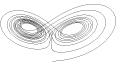
In dissipative systems, when the temporal evolution is bounded in a limited region of the phase space, a small volume should fold, after an initial stretching due to the strong sensitivity on the initial state. In presence of chaos, the competitive effect of repeated stretching and folding produces very complex and irregular structures in phase space (see an example in Transport and Diffusion). The asymptotic motion evolves on a foliated structure called a strange attractor, usually with non-integer Hausdorff dimension. In other words, strange attractors are often fractals.

In large systems, just as in small ones, the existence of a positive Lyapunov exponent (LE) is the standard criterion for chaos. In high dimensional systems besides the practical numerical difficulties one has to face with additional problems, for instance the spatial correlation, the existence of a thermodynamic limit for quantities as the whole spectrum of the Lyapunov exponents and the dimension of the attractor.

However, a chaotic extended system can be coherent (i.e. spatially ordered) or incoherent (spatially disordered).

Dynamical systems with many degrees of freedom may have many time scales, somehow related to the different scales of motion in the phase space. In contrast with systems modeled in terms of random processes, such as Langevin equations, it is not possible to separate the degrees of freedom in only two classes, corresponding to the slow and the fast modes.

In addition, even if the maximum Lyapunov exponent is negative, and the system is not chaotic, one can have a sort of "spatial complexity". This happens in the open flows in presence of the convective instability.

Let us give some paradigmatic examples of real systems with chaotic behavior:

(A) Fluid-dynamical Turbulence
(B) Chemical Turbulence. A celebrated example is the Belousov-Zhabotinsky reaction in which one has time dependence in the concentration, in the form of limit cycles or even strange attractors.
(C) Pattern formation, e.g. Turing structures.
(D) Fronts dynamics, e.g. combustion.

This kind of phenomena can be studied in terms of dynamical systems as

(A) Shell models
(B) Partial Differential Equations, as Kuramoto-Sivashinky
(C) Coupled Map Lattices (CML)
(D) Cellular Automata (CA) and CML

In the characterization of the behaviors of dynamical systems one is faced by two different cases:

(a) the evolution laws are known
(b) one has some time record from an experiment and the relevant variables are not known.

In the case (a), at least at non rigorous level and with many nontrivial exceptions, it is possible to give quantitative characterizations in terms of Lyapunov exponents, dimension of the attractor, Kolmogorov-Sinai entropy, and so on. In particular, by means of these tools one can quantify the ability to make definite predictions on the system, i.e. to give an answer to the so called predictability problem.

The case (b), from a conceptual point of view, is quite similar to the case (a). If one is able to reconstruct the phase space then the computation of quantities as Lyapunov exponent and fractal dimension can be performed basically with the same techniques of case (a). On the other hand there are rather severe practical limitations for not so high dimensional systems and even in low dimensional ones non trivial features can appear in presence of noise.

Let us remark that the mathematically well defined basic concepts (e.g. Lyapunov exponents and attractor dimension) in dynamical systems refer only to asymptotic limits, i.e. infinite time and infinitesimal perturbation. Therefore, in realistic systems, in which one typically has to deal with non infinitesimal perturbations and finite times, it is necessary to introduce suitable tools which do not involve these limits.

The standard scenario for predictability in dynamical systems can be summarized as follows. Based on the classical deterministic point of view of Laplace [1814], it is in principle possible to predict the state of a system, at any time, once the evolution laws and the initial conditions are known. In practice, since the initial conditions are not known with arbitrary precision, one considers a system predictable just up to the time at which the uncertainty reaches some threshold value D, determined by the particular needs.

In the presence of deterministic chaos, because of the exponential divergence of the distance between two initially close trajectories, an uncertainty Dx(0) on the state of the system at time t=0 typically increases as

|Dx(t)| = |Dx(0)| exp(lambda t) (1)

where lambda is the maximum Lyapunov exponent. As a consequence, starting with Dx(0)=d₀, the typical predictability time is

T_p= 1/lambda ln(D/d₀). (2)

Basically, this relation shows that the predictability time is proportional to the inverse of the Lyapunov exponent: its dependence on the precision of the measure and the threshold, for practical purposes, can be neglected.

Relation (2) is a satisfactory answer to the predictability problem only for d₀,D infinitesimal and for long times. The above written simple link between predictability and maximum Lyapunov exponent fails in generic settings of dynamical systems. Let us briefly discuss why.

The Lyapunov exponent lambda is a global quantity: it measures the average exponential rate of divergence of nearby trajectories. In general there exist finite-time fluctuations of this rate and it is possible to define an ``instantaneous'' rate: the ``effective Lyapunov exponent'' . For finite time delay tau, the effective LE depends on the particular point of the trajectory x(t) where the perturbation is performed. In the same way, the predictability time T_p fluctuates, following the variations of the effective LE.
In dynamical systems with many degrees of freedom, the interactions among different degrees of freedom play an important role in the growth of the perturbation. If one is interested in the case of a perturbation concentrated on certain degrees of freedom (e.g. small length scales in weather forecasting), and a prediction on the evolution of other degrees of freedom (e.g. large length scales), even the knowledge of the statistics of the effective Lyapunov exponent is not sufficient. In this case it is important to understand the behaviour of the tangent vector z(t), i.e. the direction along which an infinitesimal perturbation grows. In such a situation a relevant quantity can result the time, T_R, the tangent vector needs to relax on the time dependent eigenvector e₁(t) of the stability matrix, corresponding to the maximum Lyapunov exponent lambda₁. So that, in this context, one has:
T = T_R+1/lambda ln(D/d₀) (3)
and the mechanism of transfer of the error Dx through the degrees of freedom of the system, which determines T_R, could be more important than the rate of divergence of nearby trajectories.
In systems with many characteristic times -- such as the eddy turn-over times in fully developed turbulence -- if one is interested in non infinitesimal perturbations T_p is determined by the detailed process due to the nonlinear effects in the evolution equation for Dx. In this case, the predictability time could be unrelated to the maximum Lyapunov exponent and T_p might depend, in a non-trivial way, on the details of the system. Therefore one needs a new indicator, such as the finite size Lyapunov exponent (FSLE) , to characterize quantitatively the error growth of non infinitesimal perturbations.
In presence of noise, or in general of probabilistic rules in the evolution laws (e.g. random maps), there are two different ways to define the predictability: by considering either two trajectories of the system with the same noise or two trajectories of the same system evolving with different realizations of the noise. Both these definitions are physically relevant in different contexts but the results can be very different in presence of a strong dynamical intermittency.
In spatially extended systems one can have both temporal and/or spatial complex behaviour. In particular, even in absence of temporal chaos (i.e. lambda <0) one can have irregularity in the spatial features. Thus even if temporal sequences of a given site are predictable the detailed spatial structure is very ``complex'' (unpredictable). In particular, in the so called open flows (as shear flow downstream) convective instability may occur, i.e. even if the Lyapunov exponent is negative perturbations may grow in a coordinate system traveling with non zero speed. From this the necessity to define new indicators such as the co-moving Lyapunov exponent (CLE). In such situations one has the phenomenon of sensitivity on boundary conditions which can be detected by a ``spatial Lyapunov exponent''.

In the study of data sequences another approach, at first glance completely different, has been developed in the context of the information theory, data compression and algorithmic complexity theory. Nowadays it is rather clear that this approach is closely related to the dynamical systems one. Basically, if a system is chaotic, i.e. there is strong sensitivity on the initial conditions, and the predictability is limited up to a time which is related to the first Lyapunov exponent, then a time sequence obtained from one of its chaotic trajectories cannot be compressed by an arbitrary factor.

It is easy to give an interpretation of eq. (2) in terms of cost of the transmission, or difficulty in the compression, of a record x(1),x(2),......,x(N). For instance, in the discrete-time case with a unique positive Lyapunov exponent, one can show that, in the limit N--->infty, the minimum number of bits per unit time necessary to transmit the sequence is lambda/ln2. This is a rephrasing, in the context of the dynamical systems, of the theorem for the maximum compressibility which, in information theory, is stated in terms of the Shannon entropy.

On the other hand, as for the basic theoretical concepts introduced in dynamical systems theory, also in this context, in order to treat realistic problems, it is necessary to extend and generalize the fundamental notions of the information and data compression theory. In this framework perhaps the most important development has been the idea of epsilon- entropy (or rate distortion function, according to Shannon) which is the information counterpart of the finite size Lyapunov exponent.

The study of the predictability, a part its obvious interest per se and for applications (e.g. in geophysics and astronomy), can be read, from a conceptual point of view, as a way to characterize the ``complexity'' of dynamical systems.