The Manual of the initial version of Weightfield explains the basics feature of the program Manual_Weightfield.pdf

Description of the program in two pages - 1 - 2

The following pages refer to WF2 5.13

The following presentations illustrate the features of Weightfield2

1. A)N. Cartiglia, Picosecond Workshop  2018 (pdf)
   

2. B)F. Cenna, Tredi 2014, Genova (pdf)
   

3. C)F. Cenna, RESMDD14, Firenze (pdf)
   

4. D)N. Cartiglia, IEEE 2014, (poster)
   

5. E)B. Baldassarri VCI 2016, (poster)
   

The results of the simulation are displayed in these tabs:

Description of the first column:

Run Configuration

Precision: the program can track every charge, or one every 2, 3...10.

For example, if precision = 4, the program tracks 1 every 4 particles.

Time step: time interval of the simulation. 1-2 ps is ~ maximum

Output File: The currents are written to a file.

Batch Mode: allows to run many events in sequence. If Rand is checked, the impact point is chosen randomly on the detector

Select Particles

#e/h: if “uniform Q” is selected, this field allows you to set how many e/h pairs are generated

X and angle: It allows to select where the particle hits the detector and its angle.

# of particles: more than one particle per event

Rand: the position is selected randomly within the strip pitch while the angle is chosen randomly around the Angle value.

Drop down menu:

Many options, mostly self explanatory

MIP uniform Q: the energy deposition is uniform, with 75 e/h per micron

MIP non uniform, Qtot = 75*Height: the energy distribution follows locally a Landau distribution, but the overall number of charges is identical to the case above

MIP non uniform, Qtot = Landau: the energy distribution follows locally a Landau distribution, and the overall number of charges  is taken from the paper S. Meroli, D. Passeri and L. Servoli 11 JINST 6 P06013.

Alpha from top (bottom): the energy is deposited in the top (bottom) part of the detector for a length given by the Set range value

Current Pulse: the current input to the electronic simulation is given by a current pulse

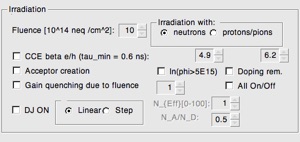
Irradiation:

CCE: Charge collection efficiency: trapping of charge carriers

Acceptor creation: standard deep p-doping level creation

ln(Phi>5E15): acceptor creation becomes logarithmic above 5E15

Doping rem: removal of initial doping (acceptor)

Gain quenching: at high fluences, the gain is quenched due to lattice defects

DJ  (Double Junction): creation of double junction due to high leakage current

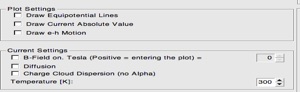
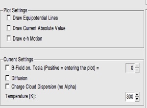
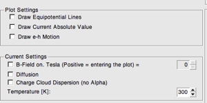
Plot Settings

Draw Electric Field: superposes to the Potential plot in the Drift Potential tab the line of equal E field.

Draw Current Absolute Value: it draws the current always positive. Note: bipolar signals look strange.

Show e/h motion: it allows to see the position of e/h in the drift 

Current Settings

Switch B-Field: adds a B field to the drift

Diffusion: adds the effect of diffusion at a given temperature

Charge Cloud Dispersion: it turns on charge cloud  effects (simplified code)

Temperature: it controls the effect of temperature on the mobility and diffusion

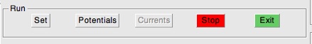
To run the program:

1. 1)First insert the values that fit your simulation,
   

2. 2)Then push the Potentials button,
   

3. 3)and then Currents.
   

4. 4)Set button: shows the geometry you have chosen