Polymer dynamics in fluids

A polymeric molecule consists in a long chain formed by the repetition of a large number of single identical units, the monomers, linked by chemical bonds. For typical polymer used in drag reductions experiments the number of monomers is very large, $N=O(10^6 - 10^7)$ and the polymer can be considered, following Kuhn, as a freely jointed chain on $n$ segments of length $b$, with independent relative orientation.

When a polymer molecule is put into an homogeneous flow, it assumes the aspect of a statistically spherical coil, because of the thermal agitation.

The average size of the coil, which is also called radius of gyration, can be estimate as the length of the random walk formed by the $n$ independent segments as $R_0 \sim n^{1/2}b$, in agreement with the results of light scattering experiments [44]. It is important to notice that the freely jointed segments do not correspond the single monomers, whose relative orientation is not independent because of the presence of chemical bonds. Indeed, for flexible linear molecules in good solvent, according to Flory[45] the radius of gyration is related to the number of monomers $N$ as:

$$R_0 = N^{3/5} a$$ (3.1)

where $a$ is the length of the single monomer. Typical value of $R_0$ are of order $0.1-0.2 \mu m$. The coiled shape must be intended in a statistical sense: it correspond to the average of all the possible configurations assumed by a polymer in an homogeneous flow, but it doesn't mean that a given polymer at a given time looks like a sphere of radius $R_0$.

On the contrary, in a inhomogeneous flow the molecule is stretched into an elongated shape, that can be characterized by its end-to-end distance $R$, which can be significantly larger than $R_0$. The deformation of the molecules is the result of the competition between the stirring exercised by the gradients of velocity, and the relaxation of the polymer to its equilibrium configuration, as a result of Brownian bombardment. Experiments with DNA molecules [46,47] show that this relaxation is linear provided that the elongation is smaller compared to the maximum extension $R \ll R_{max}$ (see Fig. 3.1).

Figure: Images from Perkins Smith & Chu, Science 264, 819 (1994) of a single DNA molecule ($~40 \mu m$) tethered to a $1 \mu m$ latex bead. The bead was trapped using optical tweezers and the DNA was labeled with a fluorescent dye. The DNA was stretched in a flow and its entropic relaxation was observed after the flow was turned off (left to right, 5 seconds intervals).

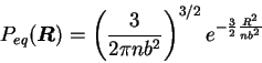
This is consistent with the freely jointed chain model, where the equilibrium distribution for the end-to-end vector $R$ resulting from the Brownian motion of the $n$ elements of the chain has a Gaussian core:

$$P_{eq}({\mbox{\boldmath$R$}}) = \left( {3 \over 2 \pi n b^2} \right)^{3/2} e^{-{3 \over 2} {R^2 \over n b^2}}$$ (3.2)

with variance $<{\mbox{\boldmath$R$}}^2> = nb^2 = 3R_0^2$. A quadratic entropy function for ${\mbox{\boldmath$R$}}$ leads, in the framework of the classical Fluctuation-Response theory [48] , to a linear relaxation $\dot{\mbox{\boldmath$R$}} = -R /\tau$.

A convenient measure on the relaxation time for the linear chain is that introduced by Zimm [49]:

$$\tau = {\mu R_0^3 \over k_B T}$$ (3.3)

where $k_B$ is the Boltzmann constant, $T$ is the solution temperature, $\mu$ is the solvent viscosity.

Indeed the relaxation process can be much more complex that the simple description given by Zimm model. Several microscopic model of the behavior of polymer molecule has been developed to characterize this process, from the Rouse chain to the Reptation model. An introduction to these models can be found in Doi & Edwards [50]. Nevertheless the simple linear relaxation is able to grasp, at least qualitatively, the basic features of polymer dynamics and feedback.

The relative strength between the relaxation of the polymer and stretching exerted by the flow is measured by the Weissenberg number $Wi$, defined as the product of the characteristic velocity gradient and $\tau$. When $Wi \ll 1$ relaxation is fast compared with the stretching time, and the polymers remain in their coiled state. On the contrary, for $Wi \gg 1$ the polymers are stretched by the flow, and they became substantially elongated. This transition is known as the coil-stretch transition, and has been demonstrated to occur under general conditions in unsteady flow[51,52] For the case of steady flow the transition is always present for purely elongational flow, while can be suppressed by rotation, because the polymers does not point always in the stretching direction[53].

In the case of turbulent flows polymers are stretched by a chaotic smooth flow, because their size is typically smaller than the viscous Kolmogorov scale of the fluid. The intensity of the stretching due to the gradients of a chaotic smooth velocity field can be measured by means of the Lyapunov exponent of Lagrangian trajectories $\lambda$ that is the average logarithmic divergence rate of nearby fluid trajectories. The Weissenberg number for chaotic smooth flow thus reads:

$$Wi = \lambda \tau$$ (3.4)

For a turbulent flow the Lyapunov exponent gives an measure of the characteristic gradients of velocity which are determined by the smallest eddies of the turbulent cascade. By dimensional arguments it can be thought of as the inverse of the fastest eddy-turnover time. Within the Kolmogorov scaling the characteristic time at viscous scale $\eta \sim \epsilon^{-1/4} \nu^{3/4}$ is given by $\tau_{\eta} \sim \epsilon^{-1/3} \eta^{2/3} \sim \epsilon^{-1/2} \nu^{1/2}$, and consequently as the Reynolds number increases, the Lyapunov exponent grows as $\lambda \sim \sqrt{Re}$ as well as the the Weissenberg number $Wi \sim \sqrt{Re}$. Thus at a critical $Re$ number the coil-stretch transition occurs.

The stretching of polymers is limited by their back reaction on the fluid. Indeed the stress tensor for a viscoelastic solution has an elastic component which is proportional to the polymer deformation tensor. When polymer are substantially elongated the elastic stresses can become of the same order of the viscous stresses, and consequently polymers can modify the flow reducing the stretching and giving rise to a dynamical equilibrium state characterized by constant average elongation, which depends on the polymer concentration.

The reduction of the stretching due to polymers back reaction correspond to a strong reduction of the Lagrangian Lyapunov exponent of the viscoelastic fluid[54,55], thus for the sake of clearness we will always define the $Wi$ number a-priori as the product of the polymer relaxation time and the Lyapunov exponent of the Newtonian fluid $Wi \equiv \lambda_N \tau$.