Phenomenology of the turbulent cascade

The basic phenomenology of turbulence can be recovered from a simple dimensional analysis of Navier-Stokes equations, using the image of the turbulent cascade proposed by Richardson [9].

The kinetic energy is supposed to be injected by an external forcing which sustains the motion of large scale eddies. This structures are deformed and stretched by the fluid dynamics, until they break into smaller eddies, and the process is repeated such that energy is transported to smaller and smaller structures. Finally at small scales the kinetic energy is dissipated by the viscosity of the fluid. The whole process of transport of energy from the large scale of injection to the small dissipative scale, through the hierarchy of eddies is known as turbulent cascade. It is worthwhile to remember that the eddies must not be thought as real vortices, but just as a metaphoric description of the triadic interaction between modes which has been formally presented in the previous section.

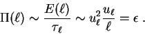
A dimensional analysis of the different terms of Navier-Stokes equation provides an estimate for the time required to transfer energy from an eddy of size $\ell$ to smaller eddies $\tau_{\ell} \sim \ell / u_{\ell}$, where $u_{\ell}$ is the rms velocity fluctuation on the scale $\ell$, and the time required to dissipate the energy contained in the same eddy by the viscous term: $\tau_\ell^{diss} \sim \ell^2 / \nu$.

Three different range of scales can thus be identified:

Injective range

which corresponds to the large scales where the forcing injects the energy.

Inertial range

where the time required for energy transfer is shorter than the dissipative time $\tau_{\ell} << \tau^{diss}_{\ell}$ and the energy is thus conserved and transported to smaller scales.

Dissipative range

where the energy dissipation overcomes the transfer and the cascade is stopped.

The hypothesis of a statistically steady state for the turbulent cascade requires a constant energy flux $\Pi(\ell)$ in the inertial range, i.e. a constant rate of energy transfer that must be equal to the energy dissipation rate $\epsilon$:

$$\Pi(\ell) \sim {E(\ell) \over \tau_{\ell}} \sim u_{\ell}^2 {u_{\ell} \over \ell} = \epsilon \;.$$ (1.42)

The above relation determines the Kolmogorov scaling for velocities and characteristic times:

$$u_{\ell} \sim \epsilon^{1/3} \ell^{1/3}$$ (1.43)

$$\tau_{\ell} \sim \epsilon^{-1/3} \ell^{2/3}$$ (1.44)

The border between the inertial and dissipative range is identified by the Kolmogorov scale $\eta$, where the dissipative and transfer times are equal $\tau_{\ell} = \tau^{diss}_{\ell}$:

$$\eta \sim \epsilon^{-1/4} \nu^{3/4}$$ (1.45)

Below the Kolmogorov scale, the viscous linear term dominates the evolution of the fluid, and the resulting velocity field is smooth and differentiable.