Energy transfer

As shown by the global energy balance (Eq. 1.16) the non-linear term in Navier-Stokes equation does not change the total kinetic energy. Nevertheless it plays a fundamental role in turbulence, because it is responsible for the energy transfer between different modes which is the origin of the turbulent cascade. To describe how it is involved in the energy transfer it is worthwhile to consider the energy balance in Fourier space. 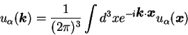For the sake of simplicity we will consider the infinite volume limit, in which the fluid is supposed to fill the entire space, and the Fourier transform reads

$$u_{\alpha}({\mbox{\boldmath$k$}}) = \frac{1}{(2 \pi)^3} \int... ...\cdot {\mbox{\boldmath$x$}}} u_{\alpha}({\mbox{\boldmath$x$}})$$ (1.18)

and its inverse is

$$u_{\alpha}({\mbox{\boldmath$x$}}) = \int d^3k e^{i {\mbox{\b... ...\cdot {\mbox{\boldmath$x$}}} u_{\alpha}({\mbox{\boldmath$k$}})$$ (1.19)

The reality condition on the velocity fields $u^{\ast}_{\alpha}({\mbox{\boldmath$x$}}) = u_{\alpha}({\mbox{\boldmath$x$}})$ in Fourier space reads $u^{\ast}_{\alpha}({\mbox{\boldmath$k$}}) = u_{\alpha}(- {\mbox{\boldmath$k$}})$, and the derivatives became multiplicative operators ( $\nabla \to i{\mbox{\boldmath$k$}}$), thus the incompressibility assumption is written as ${\mbox{\boldmath$k$}} \cdot {\mbox{\boldmath$u$}} = 0$. In Fourier space Navier-Stokes equation has the form:

$$\frac {\partial u_{\alpha} ({\mbox{\boldmath$k$}}) }{\partial t} = -i \int d^3p \ (k_{\beta} - p_{\beta}) u_{\beta} ({\mbox{\boldmath$p$}}) u_{\alpha}({\mbox{\boldmath$k$}} - {\mbox{\boldmath$p$}}) +$$

$$+ i \frac {k_{\alpha}}{k^2} \int d^3p \ p_{\gamma} (k_{\beta} - p... ...box{\boldmath$p$}}) u_{\gamma}({\mbox{\boldmath$k$}} - {\mbox{\boldmath$p$}}) +$$

$$- \nu k^2 u_{\alpha}({\mbox{\boldmath$k$}})$$ (1.20)

where it is still possible to distinguish the inertial term, the pressure term and dissipative term, while the forcing has been omitted. The constant density has been fixed to $\rho =1$.

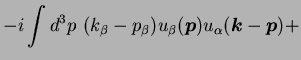
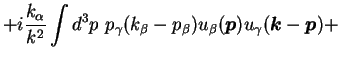
Using the incompressibility and the symmetry of the integrals for $({\mbox{\boldmath$p$}} , {\mbox{\boldmath$k$}} - {\mbox{\boldmath$p$}} ) \to ({\mbox{\boldmath$p$}} - {\mbox{\boldmath$k$}} , {\mbox{\boldmath$p$}} )$ it is possible to rewrite Eq. (1.20) as

$$\left( \frac {\partial }{\partial t} +\nu k^2 \right) u_{\al... ...$}}) u_{\gamma}({\mbox{\boldmath$k$}} - {\mbox{\boldmath$p$}})$$ (1.21)

Introducing the tensors

$$P_{\alpha \beta} ({\mbox{\boldmath$k$}}) = \delta_{\alpha \beta} - \frac {k_{\alpha} k_{\beta}}{k^2}$$ (1.22)

$$P_{\alpha \beta \gamma} ({\mbox{\boldmath$k$}}) = k_{\beta} ... ...h$k$}}) + k_{\gamma} P_{\alpha \beta} ({\mbox{\boldmath$k$}})$$ (1.23)

Navier-Stokes equation can be written in Fourier space as:

$$\left( \frac {\partial }{\partial t} +\nu k^2 \right) u_{\al... ...$}}) u_{\gamma}({\mbox{\boldmath$k$}} - {\mbox{\boldmath$p$}})$$ (1.24)

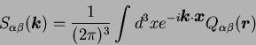
Let's now introduce some notations. The two-point correlation function is defined as

$$Q_{\alpha \beta} ({\mbox{\boldmath$r$}}) = \langle u_{\alpha... ...\beta} ({\mbox{\boldmath$x$}} + {\mbox{\boldmath$r$}}) \rangle$$ (1.25)

where $\langle \ldots \rangle$ stands for the average over the volume $V$ $\langle f({\mbox{\boldmath$x$}}) \rangle = {1 \over V} \int_V d^3x f({\mbox{\boldmath$x$}})$. Its Fourier transform is

$$S_{\alpha \beta}({\mbox{\boldmath$k$}}) = \frac{1}{(2 \pi)^3... ...{\mbox{\boldmath$x$}}} Q_{\alpha \beta}({\mbox{\boldmath$r$}})$$ (1.26)

and the correlation function in Fourier space reads

$$\langle u_{\alpha} ({\mbox{\boldmath$k$}}) u_{\beta} ({\mbox... ...mbox{\boldmath$k$}}') S_{\alpha \beta} ({\mbox{\boldmath$k$}})$$ (1.27)

The assumption of isotropy imposes for the tensor $S_{\alpha \beta}$ the form

$$S_{\alpha \beta}({\mbox{\boldmath$k$}}) = A(k) k_{\alpha} k_{\beta} + B(k) \delta_{\alpha \beta}$$ (1.28)

where $A$ and $B$ are function of the modulus $k = \vert{\mbox{\boldmath$k$}}\vert$. Multiplying Eq. (1.27) by $k_{\beta}$ and using incompressibility one gets $B(k) = -k^2 A(k)$, which substituted in Eq. (1.28) leads to

$$S_{\alpha \beta}({\mbox{\boldmath$k$}}) = P_{\alpha \beta}({\mbox{\boldmath$k$}}) B(k)$$ (1.29)

The energy spectrum is defined as the integral of the square modulus of velocity over a shell with fixed modulus $k$ in Fourier space:

$$E(k) = {1 \over 2} \int k^2 d\Omega_k \vert{\mbox{\boldmath$u$}}({\mbox{\boldmath$k$}})\vert^2$$ (1.30)

and the total energy is its integral $E = \int_0^{\infty} dk \ E(k)$. By definition $S_{\alpha \alpha} ({\mbox{\boldmath$k$}}) = \langle \vert {\mbox{\boldmath$u$}}({\mbox{\boldmath$k$}}) \vert^2 \rangle$, but from Eq. (1.29) $S_{\alpha \alpha} ({\mbox{\boldmath$k$}}) = 2 B(k)$, thus the following relation holds

$$B(k) = \frac{1}{4 \pi k^2} E(k)$$ (1.31)

which gives the relation between the energy spectrum and the Fourier transform of two-point correlation function:

$$S_{\alpha \beta} ({\mbox{\boldmath$k$}}) = \frac{E(k)}{4 \pi k^2} P_{\alpha \beta} ({\mbox{\boldmath$k$}})$$ (1.32)

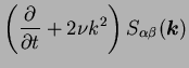
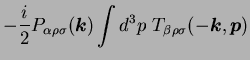
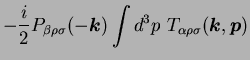
The temporal derivative of the two-point correlation function is obtained from Navier-Stokes equation as

$$\left( \frac{\partial}{\partial t} + 2 \nu k^2 \right) S_{\alpha \beta} ({\mbox{\boldmath$k$}}) = - {i \over 2} P_{\alpha \rho \sigma} ({\mbox{\boldmath$k$}}) \int d^3p \ T_{\beta \rho \sigma} (-{\mbox{\boldmath$k$}},{\mbox{\boldmath$p$}})$$

$$- {i \over 2} P_{\beta \rho \sigma} (-{\mbox{\boldmath$k$}}) \int d^3p \ T_{\alpha \rho \sigma} ({\mbox{\boldmath$k$}},{\mbox{\boldmath$p$}})$$ (1.33)

where has been introduced the three-point correlation function

$$\langle u_{\alpha} ({\mbox{\boldmath$k$}}) u_{\beta} ({\mbox... ...a \beta \gamma} ({\mbox{\boldmath$k$}},{\mbox{\boldmath$k$}}')$$ (1.34)

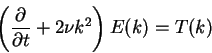
The energy balance is obtained from Eq. (1.33) remembering the relation (1.32) between the energy spectrum and the two-point correlation function. Using the antisymmetry $P_{\alpha \beta \gamma} (-{\mbox{\boldmath$k$}}) = - P_{\alpha \beta \gamma} ({\mbox{\boldmath$k$}})$ and the reality condition $T_{\alpha \beta \gamma} (-{\mbox{\boldmath$k$}},{\mbox{\boldmath$p$}}) = T^{\ast}_{\alpha \beta \gamma} ({\mbox{\boldmath$k$}},-{\mbox{\boldmath$p$}})$ on gets

$$\left( \frac{\partial}{\partial t} + 2 \nu k^2 \right) E(k) = T(k)$$ (1.35)

where has been introduced the energy transfer $T(k)$:

$$T(k) = -4 \pi k^2 k_{\rho} Im \left\{ \int d^3p \ T_{\sigma ... ...\sigma} ({\mbox{\boldmath$k$}},{\mbox{\boldmath$p$}}) \right\}$$ (1.36)

Defining the enstrophy spectrum as:

$$Z(k) = {1 \over 2} \int k^2 d\Omega_k \vert{\mbox{\boldmath$\omega$}}({\mbox{\boldmath$k$}})\vert^2 = k^2 E(k)$$ (1.37)

and restoring the external force ${\mbox{\boldmath$f$}}$ in Navier-Stoked equation, the energy balance can be rewritten as

$$\partial_{t} E(k) = -2 \nu Z(k) + T(k) + F(k)$$ (1.38)

where $F(k)$ is the injection energy spectrum:

$$F(k) = \int k^2 d\Omega_k {\mbox{\boldmath$u$}}({\mbox{\boldmath$k$}}) \cdot {\mbox{\boldmath$f$}}({\mbox{\boldmath$k$}})$$ (1.39)

If the external forcing is a Gaussian process $\delta$-correlated in time, whose statistic is determined by the correlation $\langle f_i({\mbox{\boldmath$x$}},t) f_j({\mbox{\boldmath$x$}'},t') \rangle = F(\vert{\mbox{\boldmath$x$}}-{\mbox{\boldmath$x$}'}\vert) \delta_{ij} \delta(t-t')$, the input of energy is flow-independent, i.e, the injection energy spectrum $F(k)$ is uniquely determined by the statistics of the forcing. In the case of a large scale forcing, with a forcing correlation length $L$ such that

$$F(x) \simeq F_0 for x < L$$ (1.40)

$$F(x) \simeq 0 for x > L$$ (1.41)

the injection spectrum will dominate the energy balance at small wave-numbers $k \sim k_f \sim 1/L$. On the contrary the viscous dissipation, being proportional to $\nu Z(k) = \nu k^2 E(k)$ will give strong contribution at large wave-numbers, where $k^2$ is large. In the intermediate range of wave-numbers, where both injection and dissipation of energy are negligible, the dominant term in Eq. (1.38) is the energy transfer $T(k)$. In this inertial range the energy is conserved and transferred by triadic interaction between modes with wave-numbers such that ${\mbox{\boldmath$k$}}+{\mbox{\boldmath$k$}}'+{\mbox{\boldmath$k$}}'' \simeq 0$.

Equation (1.24) for velocity involves the two-point correlation function, and Equation (1.33) for the two-point correlation function requires the tree-point one. It is easy to understand that the presence of a quadratic term in Navier-Stokes equation reproduces this closure problem at every order, i.e. the equation for the $n$-point correlation function will require the $n+1$ one. During the last fifty years several closures have been proposed, i.e. assumptions on the statistics of velocity which allow to obtain a closed set of equations for the correlation functions, from the simplest Quasi-Normal closure in which the fourth-order moments of velocity distribution are expressed in term of the second-order ones, in the same way of what happens for a Gaussian variable, to the Eddy-Damped-Quasi-Normal closure proposed by Orszag [8].