Lagrangian code for polymer dynamics

The numerical integration of viscoelastic models is rather challenging, since it is necessary to solve at the same time the modified Navier-stokes equation and the equation for the components of the conformation tensor. As a consequence, the CPU time and memory required by standard pseudospectral simulation of the viscoelastic model are about $5$ times larger in 2D than the Newtonian case with the same resolution.

Moreover the linear viscoelastic model Oldroyd-B model allows for infinite elongation, and consequently the stretching exerted by velocity gradients can generate singularities in the conformation tensor. Indeed the eigenvectors of the conformation tensor tend to align in the directions of the Lyapunov vectors, and the eigenvalues can experience exponential growth, leading to the formation of sharp fronts with diverging gradients which are involved in the feedback on the velocity fields. The consequence is a sudden rise of numerical instabilities in the simulations, which typically blow up after a short time.

Another critical aspect is the fact that the conformation tensor must remain positive definite because of its physical meaning: its eigenvalues represent the square axes of the inertia tensor. Since the smaller eigenvalues can became arbitrarily close to zero, infinitesimal errors arising from the integration scheme can bring it below zero, producing a new source of numerical instabilities.

The adoption of finite extensibility of the polymer is not sufficient to solve these problems. One of the standard trick to avoid the formation of singularities in viscoelastic simulations is the addiction of an artificial diffusivity in the equation for the conformation tensor [72]. In this way the sharp gradients are regularized, and simulations can be performed. Nevertheless this solution is not completely satisfactory, because the values of diffusivity that must be used are unrealistic, especially for passive simulations where the formation of sharp gradients is not prevented by feedback of polymers.

In order to perform accurate simulation of the passive limit for Oldroyd-B model we developed a numerical code which explicitly preserves the positive definiteness of the conformation tensor.

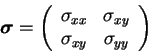
In two dimension the symmetric conformation tensor reads:

$${\mbox{\boldmath$\sigma$}} = \left( \begin{array}{cc} \sig... ... \sigma_{xy} \\ \sigma_{xy} & \sigma_{yy} \end{array}\right)$$ (A.1)

Its evolution along a Lagrangian trajectory ${\mbox{\boldmath$X$}}(s)$ is determined by the equation

$$\dot{\mbox{\boldmath$\sigma$}}({\mbox{\boldmath$X$}}(t)) = (... ...ver \tau}({\mbox{\boldmath$\sigma$}}-{\mbox{\boldmath$1$}})\;.$$ (A.2)

The velocity gradients $({\mbox{\boldmath$\nabla$} \mbox{\boldmath$u$}})_{ij}=\partial_i u_j$ are valued along the Lagrangian trajectory

$$\dot{\mbox{\boldmath$X$}}(s)={\mbox{\boldmath$v$}}({\mbox{\boldmath$X$}}(s),s) \;,$$ (A.3)

by means of standard second order interpolation of the velocity gradient fields obtained by parallel integration of Navier-Stokes equation, in which the polymer feedback has been turned off.

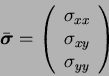
Let us write the evolution of the three components of the conformation tensor along the Lagrangian trajectory in the vectorial form:

$$\dot{\bar{\mbox{\boldmath$\sigma$}}} = {\mbox{\boldmath$A$}} \bar{\mbox{\boldmath$\sigma$}} + \bar{\mbox{\boldmath$b$}}$$ (A.4)

with:

$$\bar{\mbox{\boldmath$\sigma$}} = \left( \begin{array}{c} \sigma_{xx} \\ \sigma_{xy} \\ \sigma_{yy} \end{array}\right)$$ (A.5)

$$\bar{\mbox{\boldmath$b$}} = \left( \begin{array}{c} {2 \over \tau} \\ 0 \\ {2 \over \tau} \end{array}\right)$$ (A.6)

$${\mbox{\boldmath$A$}} = \left( \begin{array}{ccc} 2 \parti... ..._x u_y & 2 \partial_y u_y - {2 \over \tau} \end{array}\right)$$ (A.7)

The discrete evolution at first order accuracy in $dt$ can be obtained as:

$$\bar{\mbox{\boldmath$\sigma$}}(t+dt) = e^{{\mbox{\boldmath$... ...ght) - {\mbox{\boldmath$A$}}^{-1}(t) \bar{\mbox{\boldmath$b$}}$$ (A.8)

which explicitly preserves the positive definiteness of the conformation tensor. This procedure can be immediately extended to higher order integration schemes. In our simulation we have adopted a Runge Kutta second order scheme which requires a further evaluation of the matrix ${\mbox{\boldmath$A$}}$ in the mid-point ${\mbox{\boldmath$X$}}(t+dt/2)$.

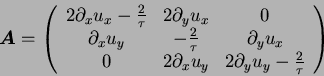
To obtain an explicit form for the exponential matrix $e^{{\mbox{\boldmath$A$}}(t)dt}$ it is necessary to distinguish the case in which the predominant effect of velocity gradients on the conformation tensor is either the stretching or the rotation, depending on the sign of the determinant of velocity gradients:

$$\det ({\mbox{\boldmath$\nabla$}}{\mbox{\boldmath$u$}}) = \partial_x u_x \partial_y u_y - \partial_y u_x \partial_x u_y$$ (A.9)

Indeed since the trace of the velocity gradients tensor vanishes because of incompressibility, the two eigenvalues must be opposite and either real, when $\det ({\mbox{\boldmath$\nabla$}}{\mbox{\boldmath$u$}}) < 0$ or pure imaginary when $\det ({\mbox{\boldmath$\nabla$}}{\mbox{\boldmath$u$}}) > 0$. In the first case, which corresponds to regions of intense stretching, the linearized flow is hyperbolic, while the second case corresponds to elliptic regions where rotation is the predominant effect.

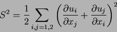
Introducing the Weiss function Q defined as [81]

$$Q = S^2 - \omega^2 = - 4 \det ({\mbox{\boldmath$\nabla$}}{\mbox{\boldmath$u$}})$$ (A.10)

where $\omega$ is the vorticity and

$$S^2 = {1 \over 2} \sum_{i,j = 1,2} \left( {\partial u_i \over \partial x_j} + {\partial u_j \over \partial x_i} \right)^2$$ (A.11)

the three cases can be distinguished according to the sign of $Q$:

hyperbolic regions

where $Q > 0$

elliptic regions

where $Q < 0$

neutral regions

where $Q = 0$