Oldroyd-B model

In the dumbbell model the behavior of a single polymer molecule in a fluid is considered, but this microscopic model doesn't describe the feedback that polymers have on the flow. To include the feedback effect it is necessary to move to an hydro-dynamical description for the viscoelastic fluid. Oldroyd-B model [57] provides a simple linear viscoelastic model for dilute polymer solutions, based on the dumbbell model.

The passage from the microscopic behavior of the single molecule to a macroscopic hydro-dynamical description requires to get rid of the microscopic degrees of freedom such as the thermal noise. The macroscopic polymer behavior can be described in term of the conformation tensor:

$$\sigma_{ij} = R_0^{-2} \langle R_{i}R_{j} \rangle$$ (3.19)

where the average is taken over thermal noise, or equivalently over a small volume $V$ containing a large number of molecules. By construction the tensor ${\mbox{\boldmath$\sigma$}}$ is symmetric, positive definite, and its trace $\textrm{tr}{\mbox{\boldmath$\sigma$}}$ is a measure of the square polymer elongation.

The equation for the conformation tensor follows from the linear equation (3.9) for the single molecule:

$$\partial_t {\mbox{\boldmath$\sigma$}} + ({\mbox{\boldmath$u$... ...ver \tau}({\mbox{\boldmath$\sigma$}}-{\mbox{\boldmath$1$}})\;,$$ (3.20)

where $\tau$ is the polymer relaxation time defined by Eq. (3.10), the matrix of velocity gradients is defined as $({\mbox{\boldmath$\nabla$} \mbox{\boldmath$u$}})_{ij}=\partial_i u_j$. The conformation tensor has been normalized with the equilibrium length $R_0$ such that in absence of external flow it relaxes isotropically to the unit tensor ${\mbox{\boldmath$1$}}$.

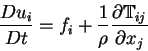
Equation (3.20) must be supplemented by the equation for the velocity field, which is derived from the momentum conservation law:

$${D u_i \over Dt} = {f_i} + {1 \over \rho} {\partial \mathbb{T}_{ij} \over {\partial x_j}}$$ (3.21)

where ${\mbox{\boldmath$f$}}$ is sum of the body forces per unit mass, and $\mathbb{T}$ is the stress tensor of the fluid.

The stress tensor of a Newtonian fluid is linear in the deformation tensor $e_{ij} = 1/2 (\nabla_j u_i + \nabla_i u_j)$, and is given by [4]:

$$\mathbb{T}_{ij}^N = -p\delta_{ij} + \mu \left[ (\nabla_j u_i + \nabla_i u_j) - {2 \over 3} \nabla_k u_k \delta_{ij} \right]$$ (3.22)

where $\mu$ is the dynamic viscosity and $p$ the static pressure.

In the case of a viscoelastic solution, the stress tensor is given by the sum of the Newtonian stress tensor $\mathbb{T}^N$ and the elastic stress tensor $\mathbb{T}^P$, which takes into account the elastic forces of the polymers. While for a Newtonian fluid the stress tensor is proportional to the deformation rate tensor via the viscosity, in the Hookean approximation for the single polymer the elastic stress tensor is proportional via the Hook modulus to the deformation tensor $T_{ij} = K_0 R_i R_j$. The elastic stress tensor per unit volume of fluid is obtained summing the average contribution given by each polymer:

$$\mathbb{T}_{ij}^P = n K_0 < R_i R_j > = n K_0 R_0^2 \sigma_{ij}$$ (3.23)

where $n$ is the concentration of polymer molecules.

For an incompressible fluid ( $\nabla \cdot {\mbox{\boldmath$u$}} = 0$) with constant density $\rho$ the equation obtained from the momentum conservation law (3.21) with the stress tensor $\mathbb{T}= \mathbb{T}^N + \mathbb{T}^P$ reads:

$$\partial_t {\mbox{\boldmath$u$}} + ({\mbox{\boldmath$u$}}\cd... ...abla$}}\cdot{\mbox{\boldmath$\sigma$}} + {\mbox{\boldmath$f$}}$$ (3.24)

where $p$ is the pressure, ${\mbox{\boldmath$f$}}$ is the external force (per unit mass) driving the flow. The solvent kinematic viscosity is denoted by $\nu = \mu / \rho$ and $\eta$ is the zero-shear contribution of polymers to the total solution viscosity $\nu_{t}=\nu(1+\eta)$:

$$\eta = {n K_0 R_0^2 \tau \over 2 \mu}$$ (3.25)

Eq. (3.24) is a generalization of Navier-Stokes equation for the viscoelastic solution and together with Eq. (3.20) fully determines the dynamics of Oldroyd-b model.