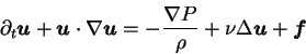
The dynamics of an incompressible Newtonian fluid is determined
by the celebrated Navier-Stokes equations (1823), supplemented by the
incompressibility condition:
Let us briefly describe the different terms in Navier-Stokes equation:
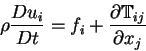
The origin of Eqs. (1.1,1.2) is just the
conservation of mass and momentum per unit volume:
The incompressibility assumption is consistent until velocities smaller
than speed of sound ![]() in the fluid are considered.
Since eventual density fluctuations are swept away exactly as sound waves,
for small value of the Mach number
which measures the ratio between the typical velocities and
the speed of sound in the considered fluid, the density can be
assumed to be constant in time and space
in the fluid are considered.
Since eventual density fluctuations are swept away exactly as sound waves,
for small value of the Mach number
which measures the ratio between the typical velocities and
the speed of sound in the considered fluid, the density can be
assumed to be constant in time and space
![]() and the mass conservation (1.4) leads to the
divergence-less condition on the velocity field
and the mass conservation (1.4) leads to the
divergence-less condition on the velocity field
![]() .
It is common to assume the constant density to be equal to unity,
or equivalently to consider dynamical quantities per unit mass of fluid.
As an example we will often refer to the square modulus of velocity as
kinetic energy.
.
It is common to assume the constant density to be equal to unity,
or equivalently to consider dynamical quantities per unit mass of fluid.
As an example we will often refer to the square modulus of velocity as
kinetic energy.
Because of the presence of a non-linear term in Navier-Stokes equation, the space of its solutions does not have an affine structure, and consequently a generic solution can not be obtained as linear superposition of basic solutions. Moreover, a typical feature of turbulence is the presence of chaos, i.e. the Navier-Stokes equations display a strong sensitivity to initial conditions, which drastically reduces the interest for their exact solutions. For this reason the theory of turbulence has a statistical approach, trying to predict the statistical properties of the flow instead of searching a peculiar analytic solution.
![\begin{displaymath}
\mathbb{T}_{ij}^N = -P\delta_{ij} +
\mu \left[ (\nabla_j u_...
...nabla_i u_j) -
{2 \over 3} \nabla_k u_k \delta_{ij} \right]\;.
\end{displaymath}](img81.png)